Overview

Remember Regression means a Relation

Linear regression is a statistical approach to analyzing and modeling the relationship between two variables, usually called the dependent variable and the independent variable, using a linear equation.

The independent variable is used to estimate or predict the value of the dependent variable. Linear regression is commonly used for making predictions based on the relationship between variables.

The regression method evaluates two main aspects. The first is whether a set of independent variables can predict the dependent variable, and the second is which independent variables have a significant impact on the outcome variable.

Introduction

Regression analysis is a type of machine learning algorithm that is used to predict continuous variables based on labeled data. It is important to choose the right type of regression method depending on your data and the problem you are trying to solve.

The linear regression model involves a single parameter and a linear relationship between the dependent and independent variables. When there is more than one independent variable, multiple linear regression models are used. The basic equation for linear regression is:

y = ax + c + e

Here, 'a' represents the slope of the line, 'c' is the intercept, and 'e' is the error in the model.

Hypothesis Function

The hypothesis function is an essential part of linear regression, which is used when there is only one independent variable and one dependent variable. The function estimates the relationship between the variables using the following formula:

Y = β0 + β1x

Here, Y represents the predicted response value, β0 is the y-intercept when x is zero, β1 is the average change in Y when x is increased by one unit, and x is the value of the predictor variable.

In simple linear regression, the null hypothesis is that there is no significant linear relationship between the independent and dependent variables. The alternative hypothesis is that there is a significant linear relationship between the variables. These hypotheses are important for determining the statistical significance of the regression model.

The following null and alternative hypotheses are used in simple linear regression:

H0: β1 = 0
HA: β1 ≠ 0

According to the null hypothesis, coefficient β1 is equal to zero. In other words, the predictor variable x and the responder variable y have no statistically relevant correlation.

β1 is not equal to zero, according to the alternative hypothesis. In other words, x and y have a statistically significant association.

We may use multiple linear regression to evaluate the connection between the variables when there are numerous independent factors and one result variable:

Y = β0 + β1x1 + β2x2 + ... + βk*xk

where:

Y: The response value that has been estimated.
β0: When all predictor variables are equal to zero, the average value of Y is 0.
βi: The average change in y when xi is increased by one unit.
xi: The xi predictor variable's value.

The following null and alternative hypotheses are used in multiple linear regression:

H0: β1 = β2 = ... = βk = 0

HA: β1 = β2 = ... = βk ≠ 0

The null hypothesis says that all of the model's coefficients are zero. In other words, there is no statistically significant association between any of the predictor factors and the response variable, y. According to the alternative hypothesis, not all coefficients are equal to zero at the same time.

Getting confused? Try to Understand Basics!

Imagine you have a graph with two axes, one is for your independent variable (which is something you can control or measure, like time or distance), and the other is for your dependent variable (which is something that changes based on the independent variable, like speed or temperature).

When we draw a straight line on this graph, it helps us understand how the dependent variable changes when we change the independent variable. And we use the equation y = mx+c to represent this line, where y is the dependent variable, x is the independent variable, m is the slope of the line (which tells us how much y changes when x changes), and c is the y-intercept (which tells us the value of y when x is 0).

Using this equation helps us make predictions about the dependent variable based on the independent variable. For example, if we know that for every increase in x by 1, y increases by 2 (which means m=2), and that when x is 0, y is 5 (which means c=5), then we can predict that when x is 3, y will be 11 (because y = 2x + 5).

This equation is really useful because it helps us understand how two variables are related and make predictions based on that relationship.

Types of Linear Regression

1. Simple Linear Regression

2. Multiple Linear Regression

Simple Linear Regression

In basic linear regression, we want to understand how one thing affects another. Specifically, we want to see how a single independent variable (like the number of hours studied) relates to a dependent variable (like the score on a test). We use an equation, Y = mx+c, to express this relationship.

In this equation, Y represents the dependent variable (like the test score), m represents the slope of the line (how much Y changes for each change in the independent variable), x represents the independent variable (like the number of hours studied), and c represents the y-intercept (where the line crosses the Y axis).

For example, let's say we want to predict a person's weight based on their height. We can collect data on 2000 people, measure their height and weight, and use linear regression to find the equation that best describes the relationship between the two variables.

Multiple Linear Regression

Multiple linear regression (MLR) is a statistical technique used to predict the outcome of a response variable based on several different factors. MLR helps to understand how the different independent variables are related to the dependent variable. It is an extension of ordinary least-squares (OLS) regression that allows for the inclusion of multiple explanatory variables.

For instance, suppose an analyst wants to know how different factors affect the sales of a product. The analyst can use MLR to determine how factors such as price, advertising expenditure, and competition impact sales. In this case, sales would be the dependent variable, and the other factors would be independent variables.

The use of MLR helps to determine which factors have a significant impact on the outcome and which ones do not. By understanding the relationship between the independent and dependent variables, the analyst can make informed decisions to improve the product's sales performance.

In summary, multiple linear regression is a statistical approach that helps to predict the outcome of a response variable based on several different independent variables. It is a useful tool in many areas, including economics, marketing, and social sciences, where the relationships between variables are often complex.

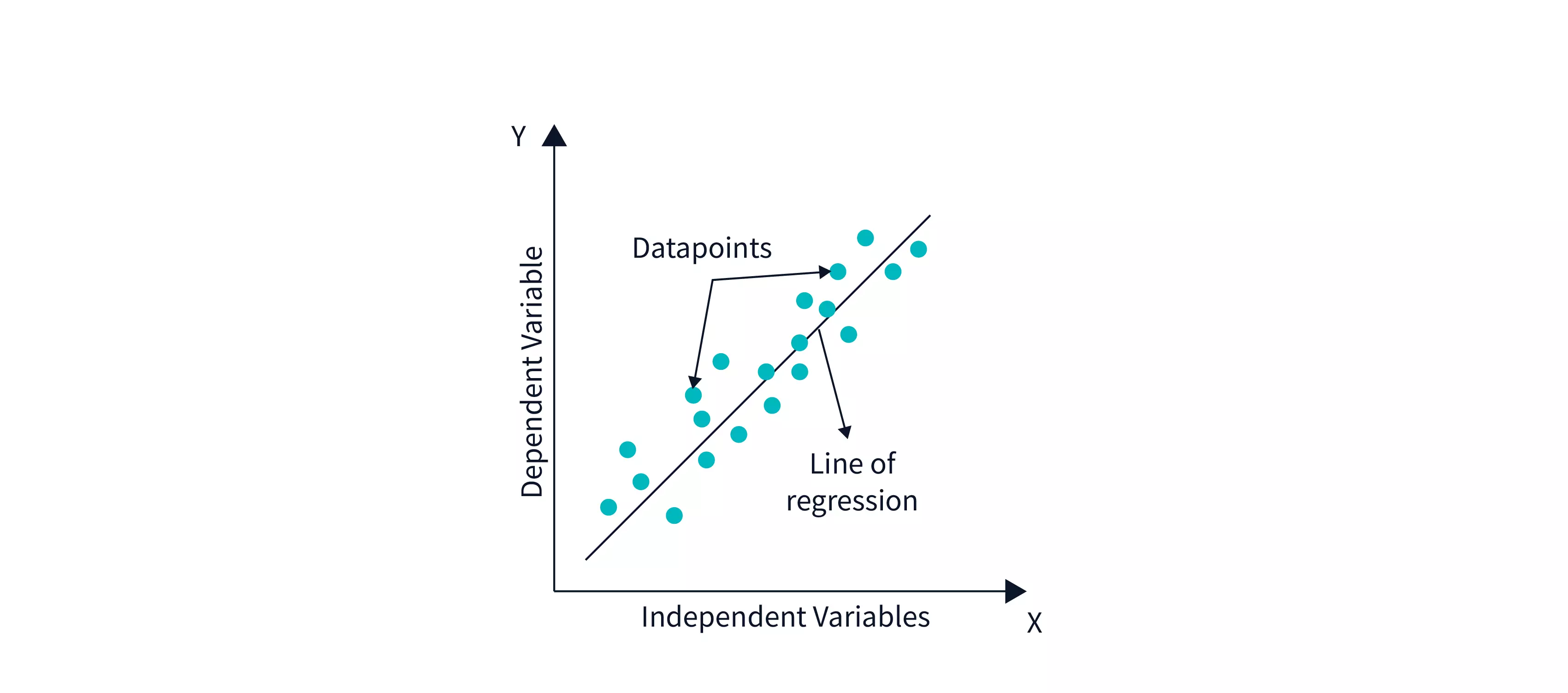
Linear Regression Line

A regression line is a straight line that depicts the connection between the dependent and independent variables. There are two sorts of relationships that may be represented by a regression line:

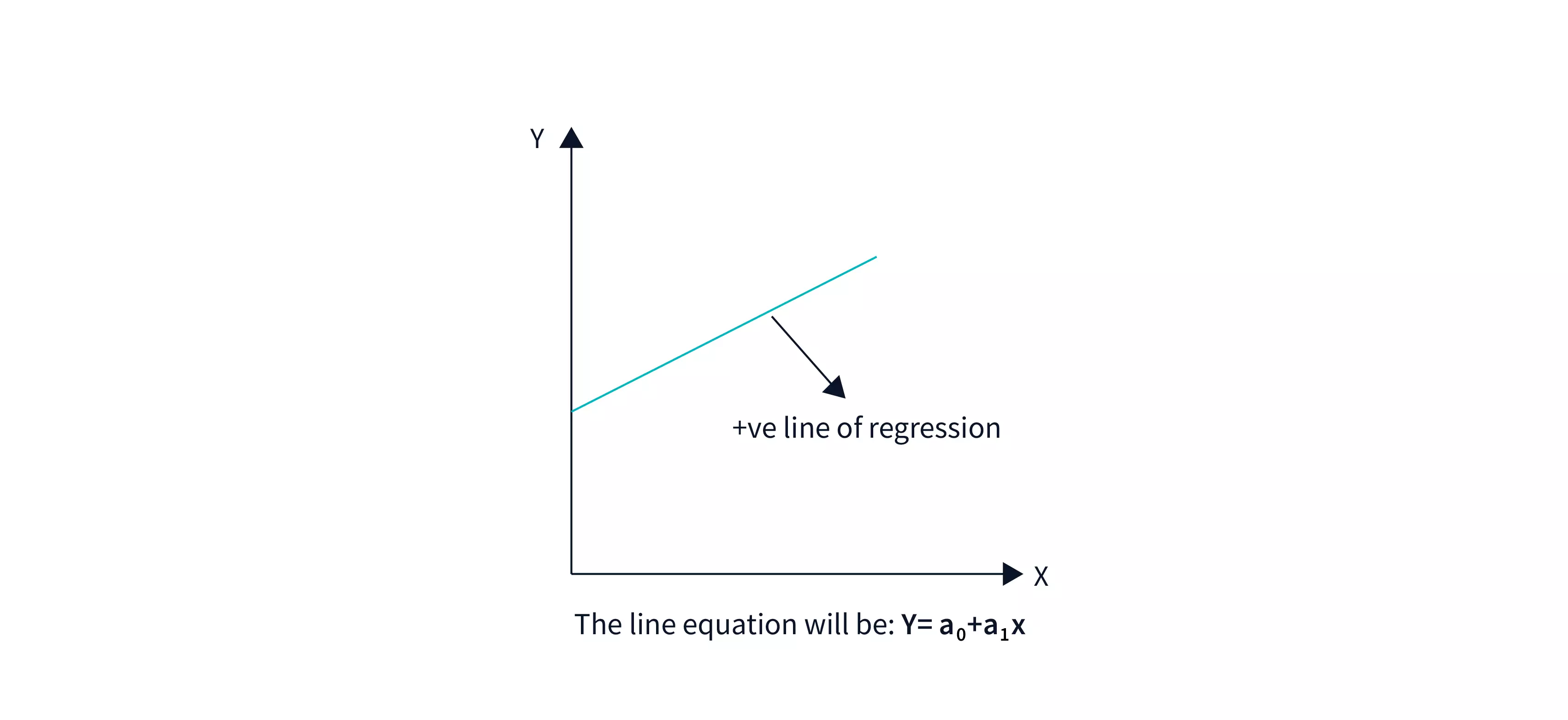
Positive Linear Correlation

A positive linear connection exists when the dependent variable rises on the Y-axis while the independent variable increases on the X-axis.

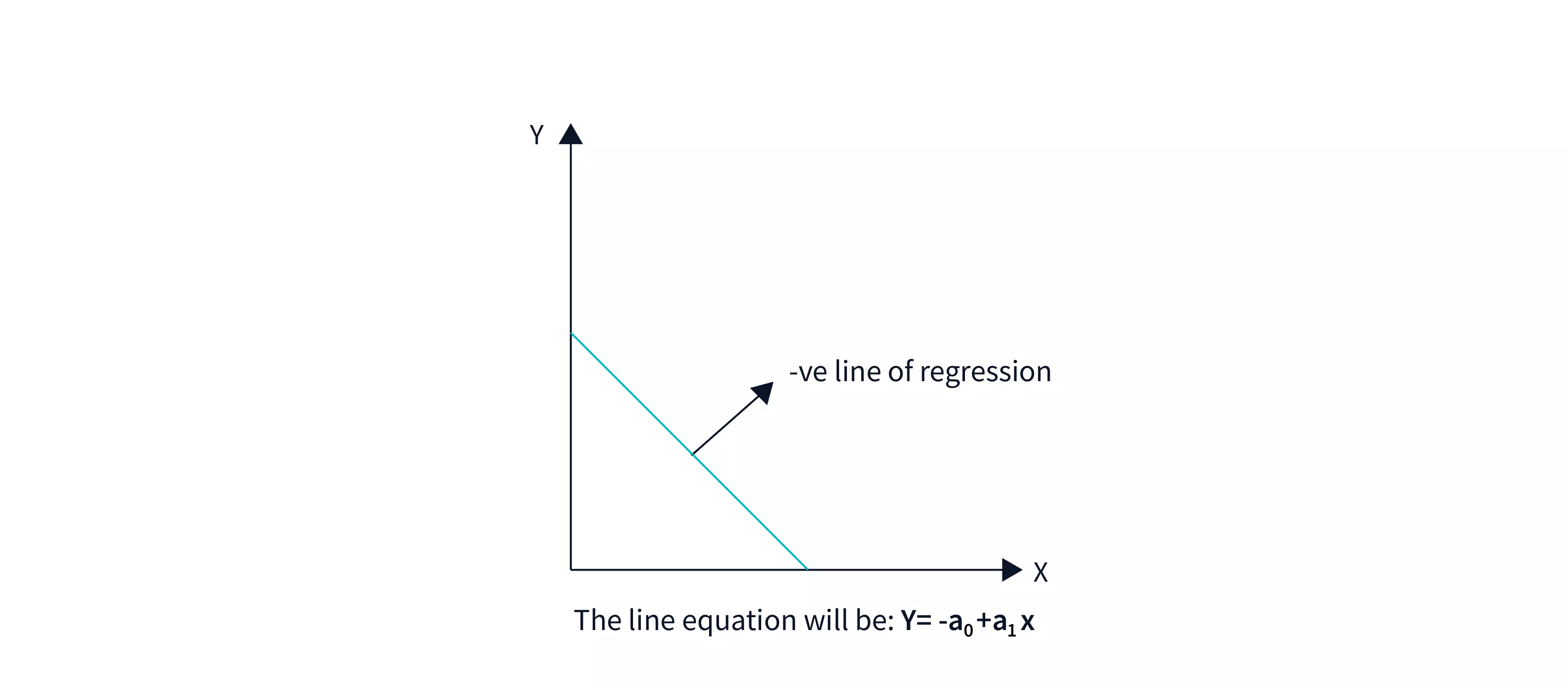
Negative Linear Correlation

A negative linear relationship exists when the dependent variable declines on the Y-axis while the independent variable grows on the X-axis.

The Best Fit Line

Imagine you're trying to draw a line that goes through a bunch of dots on a graph. You want the line to be as close to all the dots as possible. That line is called the "Best Fit Line"!

Now, the reason we want to draw this line is that it helps us understand the relationship between two things. For example, if we're looking at a graph of how much people exercise and how much weight they lose, we can draw a Best Fit Line to see if there's a connection between the two. If the line slopes downwards, it means that people who exercise more tend to lose more weight. If the line is flat, there may not be much of a connection.

So, how do we find the Best Fit Line? Well, we use a fancy math formula called "linear regression". This formula helps us figure out the equation of the line that comes closest to all the dots on the graph. It takes into account the distance of each dot from the line and tries to minimize that distance.

Once we have the equation of the Best Fit Line, we can use it to make predictions! We can plug in values for one variable (like exercise) and use the equation to predict the value of the other variable (like weight loss).

Cost Function

When we're trying to find the Best Fit Line for a set of data points, we need to figure out the values of β0 and β1. These values determine the equation for the line. But how do we know what values of β0 and β1 will give us the best line?

That's where the cost function comes in. It's like a coach who's helping us find the best values for β0 and β1. The coach wants us to get as close as possible to the actual data points, so it tells us to minimize the difference between our predictions and the real values.

To do this, we use a special formula called the Mean Squared Error (MSE) function. This formula takes the difference between each predicted value and the actual value, squares it (to get rid of negative signs), add them all up, and divides it by the total number of data points.

The result is the average squared error across all of the data points. This tells us how far off our line is from the actual data. Our goal is to adjust the values of β0 and β1 so that the MSE value reaches the minima, which means we have the best possible line.

The cost function is like a GPS that guides us toward the best-fit line for our data points. It tells us the distance between our predicted line and the actual data points. Our goal is to minimize that distance and get as close as possible to the data points. Think of it like driving towards a destination - the GPS tells us the distance we have to travel, and we keep adjusting our route until we arrive at our destination. In the same way, we adjust the values of β0 and β1 until we reach the minimum MSE value and get the best possible fit line for our data.

That's the end of the article Readers!

Will be explaining more in the following blogs!

"Two things are infinite: the universe and human stupidity; and I'm not sure about the universe." - Albert Einstein

Keep your curiosity alive and do follow me for more such Articles! 😃