Statistical Distributions

Let’s understand what is Statistical Distribution:

A key idea in statistics is statistical distributions. Making predictions and analyzing data, as well as testing hypotheses, are all made possible by them. It would be challenging to evaluate the findings of statistical analyses or derive meaningful inferences from data without a solid understanding of statistical distributions. Statistical distributions are a way of describing how data is spread out. They tell us the likelihood of different outcomes or values occurring.

There are broadly two categories of Statistical Distributions, which are

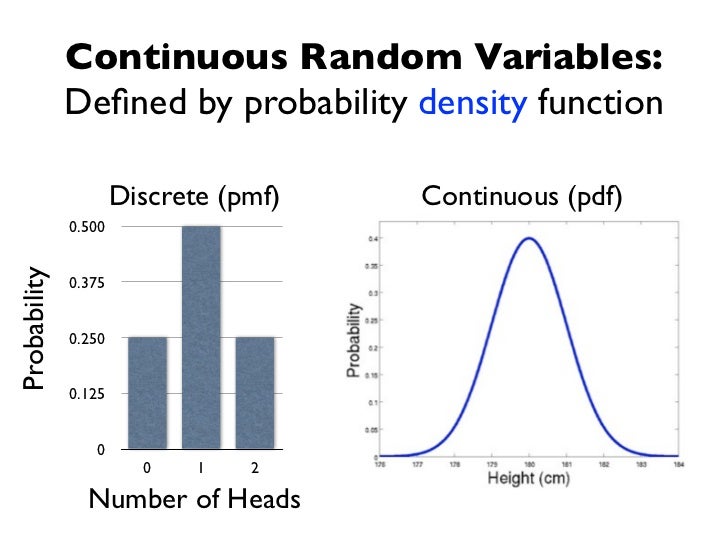
1. Discrete Statistical distribution

2. Continuous Statistical distribution

To get a brief overview of these statistical distributions, let me provide a brief outline of the two kinds of Statistical Distributions.

Discrete Statistical Distribution

1. Data that can only have a limited or countable set of numbers are the focus of discrete statistics.

2. Includes counting or tabulating statistics a lot.

3. The spread of data is represented using the probability mass function.

4. The geometric distribution, Poisson distribution, and binomial distribution are some examples.

5. Commonly employed in industries like engineering, banking, and epidemiology

6. Useful for analyzing data with a narrow spread of values or outcomes, like counts of occurrences or events

A discrete distribution is a probability distribution that describes the probabilities of a finite number of outcomes from a random variable. For example, when rolling a fair six-sided die, the possible outcomes are 1, 2, 3, 4, 5, or 6, and the probability of each outcome is 1/6.

Here's a code snippet to represent the probabilities of each outcome of rolling a fair six-sided die using Python:

# probability mass function (PMF) for rolling a six-sided die
PMF = {1: 1/6, 2: 1/6, 3: 1/6, 4: 1/6, 5: 1/6, 6: 1/6}

# calculate the probability of rolling a 3
P_3 = PMF[3]
print("The probability of rolling a 3 is:", P_3)

In this example, we create a dictionary called PMF that represents the probability mass function (PMF) of rolling a six-sided die. The keys of the dictionary represent the possible outcomes (1, 2, 3, 4, 5, or 6), and the values represent the probability of each outcome occurring. The P_3 variable represents the probability of rolling a 3, which is accessed using the key 3 in the PMF dictionary.

Now let's say we roll the die twice and want to calculate the probability of getting a sum of 7. We can use the PMF to calculate the probability of each possible outcome, and then sum up the probabilities of the outcomes that add up to 7:

# Calculate the probability of rolling a sum of 7
P_sum7 = 0
for i in range(1, 7):
    for j in range(1, 7):
        if i + j == 7:
            P_sum7 += PMF[i] * PMF[j]

print("The probability of rolling a sum of 7 is:", P_sum7)

In this example, we use two nested loops to iterate through all possible combinations of rolling the die twice. The if statement checks whether the sum of the two rolls is equal to 7, and if so, it multiplies the probabilities of the two outcomes together and adds the result to the P_sum7 variable. Finally, we print the value of P_sum7, which represents the probability of rolling a sum of 7.

Continuous Statistical Distributions

1. Continuous Data that can have any value within a range are the basis of Continuous statistical distribution

2. It utilizes data for planning and measurement

3. The spread of data is represented using the probability density function.

4. The normal distribution, exponential distribution, and chi-square distribution are some examples.

5. It is widely employed in disciplines like physics, biology, and finance

6. Analyzing data that can have a broad range of values, such as measurements of time, distance, or temperature, is made possible by this technique.

A continuous statistical distribution refers to a type of probability distribution where the random variable can take on any value within a specific range. This is in contrast to a discrete distribution, where the variable can only take on a limited set of values.

One example of a continuous distribution is the normal distribution, also known as the bell curve. This distribution is often used to model real-world phenomena such as heights, weights, and test scores.

Here's an example code in Python to generate random samples from a normal distribution with mean 0 and standard deviation 1:

import numpy as np

samples = np.random.normal(0, 1, size=1000)

This code uses the numpy library to generate 1000 random samples from a normal distribution with mean 0 and standard deviation 1. The resulting samples can take on any value within the range of the distribution, which in this case is from negative infinity to positive infinity.

In Continuous and Discrete Statistical Distributions, we have several types of distributions as I gave a few examples above. So, to just make you all a bit more familiar with the distributions you can just go through the explanations below.

Additional points to know

Continuous Distributions

Normal distribution: A commonly used bell-shaped continuous probability distribution that is often used to represent many natural phenomena.

Uniform distribution: A continuous probability distribution in which all values within a certain range have an equal chance of occurring.

Exponential distribution: A continuous probability distribution that is typically used to model the time intervals between rare events.

Beta distribution: A continuous probability distribution that is frequently used to model probabilities or proportions.

Gamma distribution: A continuous probability distribution that is commonly used to model waiting times or survival data.

Discrete Distributions

Binomial distribution: A discrete probability distribution that is often used to model the number of successes in a fixed number of independent trials.

Poisson distribution: A discrete probability distribution that is often used to model the number of rare events in a fixed interval of time or space.

Geometric distribution: A discrete probability distribution that is often used to model the number of trials needed to achieve the first success in a series of independent trials.

Hypergeometric distribution: A discrete probability distribution that is often used to model the probability of drawing a certain number of items from a population without replacement.

That's the end of the article readers!

Will be explaining more in my following blogs!

"Statistical thinking will one day be as necessary for efficient citizenship as the ability to read and write." - H.G. Wells

Do subscribe and keep supporting! 😊